
헤매어도 한 걸음씩
Uber가 딥러닝 모델을 사용하여 도착시간을 예측하는 방법 본문
DeepETA: How Uber Predicts Arrival Times Using Deep Learning
Uber가 도착시간을 예측하기 위해 왜 딥러닝 모델로 넘어가게 되었는지 알 수 있는 글이다.
아래 본문은 이를 읽고 정리한 내용이다.

우버는 사용자에게 차량 도착 예측 시간(ETA)을 제공한다.
ETA를 사용하여 요금을 계산하고, 픽업 시간을 추정하고, 라이더와 기사를 연결하고, 배송을 계획하는 등의 작업을 수행하며, 이를 정확하게 추정하는 능력은 매우 중요하다. 정확한 ETA 추정은 고객에게 긍정적인 경험을 제공하고, 서비스 가격과 운전 경로 등을 설정하는 데도 활용된다.
이 글에선 우버가 ETA 예측 개선을 위해 왜 딥러닝 모델을 선택했고, 어떤 기술을 사용했는지 다룬다.
전통적인 ETA 엔진은 도로 네트워크을 작은 세그먼트로 나눠서 그래프에 가중치를 두고 계산한다.
최단경로 알고리즘으로 최적의 경로를 찾고, ETA를 도출하기 위해 가중치를 합산한다.
하지만 지도는 지형이 아니다. 도로 그래프는 모델일 뿐이며, 실제 지형 상황을 반영하지 못한다. 또한 라이더/드라이버들이 목적지까지 어떤 경로를 선택할지 알 수 없다.
과거 데이터와 실시간 신호가 결합된 데이터를 사용하여 도로 그래프 예측 위에 머신 러닝(ML) 모델을 훈련시킴으로서ETA를 개선시킬 수 있었다.
By training machine learning (ML) models on top of the road graph prediction using historical data in combination with real-time signals, we can refine ETAs that better predict real-world outcomes.
몇 년간 우버는 ETA 개선을 위해 Gradient-boosted decision tree ensembles을 사용했지만, 이제 Apache Spark + XGBoost로는 Data와 Model을 더 늘릴 수 없는 한계에 도달한다.
→ 모델을 계속 확장하고 정확도를 개선하기 위해 데이터 병렬 SGD를 사용하여 대규모 데이터 세트로 확장하는 것이 상대적으로 쉬운 딥러닝을 선택한다.
딥러닝으로의 전환을 위해 세 가지 주요 문제점을 해결해야 했다.
- Latency : 몇 밀리초 내에 ETA 계산
- Accuracy : MAE(Mean Absolute Error, 평균 절대 오차)를 XGBoost 모델보다 개선
- Generality : 우버의 모든 비즈니스에서 전 세계적으로 ETA 예측을 제공
이러한 문제를 해결하기 위해 Uber AI는 DeepETA라는 프로젝트에서 Uber의 지도 팀과 협력하여 글로벌 ETA 예측을 위한 low-latency deep neural network architecture를 개발한다.
7가지의 신경망 아키텍처를 테스트
→ 최종적으로 Self-Attention을 이용한 Encoder-Decoder Architecture(Transformer-based)가 가장 정확했다.
트랜스포머 기반 인코더가 최고의 정확도를 제공했지만 온라인 실시간 서비스를 위한 대기 시간 요구 사항을 충족하기에는 너무 느렸다.
→ 계산을 빠르게 개선한 Linear Transformer를 선택
More Embeddings, Fewer Layers
→ DeepETA를 빠르게 하기 위해 추가적으로 feature sparsity 활용 > 기능 희소성..? 이부분은 잘 이해가 되지 않는다.
- 해당 부분 발췌
First of all, the model itself is relatively shallow with just a handful of layers. The vast majority of the parameters exist in embedding lookup tables. By discretizing the inputs and mapping them to embeddings, we avoid evaluating any of the unused embedding table parameters.
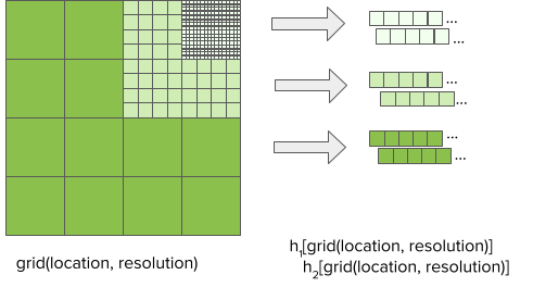
Discretizing the inputs gives us a clear speed advantage at serving time compared to alternative implementations. Take the geospatial embeddings pictured in Figure 5 as an example. To map a latitude and longitude to an embedding, DeepETA simply quantizes the coordinates and performs a hash lookup, which takes O(1) time. In comparison, storing embeddings in a tree data structure would require O(log N) lookup time, while using fully-connected layers to learn the same mapping would require O(N2) lookup time. Seen from this perspective, discretizing and embedding inputs is simply an instance of the classic space vs time tradeoff in computer science: by precomputing partial answers in the form of large embedding tables learned during training, we reduce the amount of computation needed at serving time.
출처 : https://eng.uber.com/deepeta-how-uber-predicts-arrival-times/


